www.seeingstatistics.com

Start > Differences > Categorical DV > Continuous IV or Two+ Categorical IVs: Logistic Regression

Logistic Regression

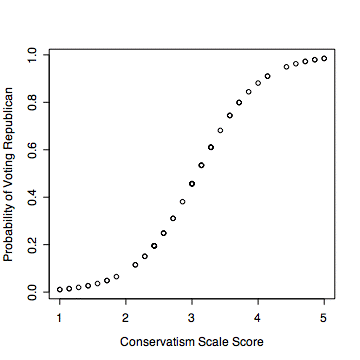
The appropriate statistical test is logistic regression. Instead of modeling the probability of the response, logistic regression models the log odds or logit, which equals log(p/(1-p)). This solves various distributional problems and ensures that when the predicted values are converted back to probabilities they will all be between 0 and 1.

Example

We will consider two examples, one with raw data and a continuous predictor variable and one with tabulated data and a categorical predictor variable.

1. The available data are scores on a scale of conservatism (the average of a number of attitude statements on a 1 to 5 scale, with 5 indicating more conservatism) and whether or not the person voted for the Republican candidate for president in the election.
2. We will use the same data from the Vail water problem used to illustsrate chi-square contingency table. For the details, see Two-Way ChiSquare.

Summary

1. Scores on a conservatism scale significantly predict the probability of voting for the Republican presidential candidate (Wald Chi-sq(1) = 14.44, p = .0001). The relationship is fairly strong with R-sq = .4. In the graph of predicted probabilities, the likelihood of voting Republican clearly increases as the conservatism score increases. Specifically, for each one-point increase on the conservatism scale the odds of voting Republican increase by a factor of about 8.8. The basic relationship is, of course, not surprising. However, the magnitude of the effect (the odds of voting Republican increase by a factor of about 8.8, 95% CI: [3.4, 33.4]) shows that the relationship is dramatic.
2. In a mountain community afflicted by a wide spread intestinal disorder, those drinking tap water were significantly more likely to be sick than those drinking bottled water (Wald ChiSq(1) = 12.63, p = .0004). The odds of being sick were six times greater for those drinking tap water (odds = 6.13, 95% CI: [2.4, 18.1]). This strongly suggests that the water treatment plant should be examined for a possible problem.

Computer Examples

R

1. Example with Raw data

The data are available in the file voting.dat.

> vote <- read.table('voting.dat',header=T)
> names(vote)
[1] "conserv" "voterep"
> attach(vote)
>vote   # note that 1 = vote republican, 0 otherwise
   conserv voterep
1    1.000       0
2    1.000       0
3    1.143       0
4    1.143       0
5    1.285       0
6    1.429       0
7    1.429       0
8    1.571       0
9    1.714       0
10   1.714       0
11   1.857       0
12   2.143       0
13   2.143       0
14   2.286       0
15   2.286       1
16   2.429       0
17   2.429       0
18   2.429       0
19   2.429       0
20   2.429       0
21   2.429       1
22   2.429       0
23   2.571       0
24   2.571       0
25   2.571       1
26   2.714       1
27   2.714       0
28   2.857       0
29   3.000       1
30   3.000       0
31   3.000       0
32   3.000       1
33   3.000       1
34   3.000       0
35   3.000       0
36   3.143       1
37   3.143       1
38   3.143       0
39   3.143       1
40   3.286       0
41   3.286       1
42   3.286       1
43   3.286       1
44   3.286       0
45   3.429       0
46   3.571       1
47   3.571       1
48   3.571       1
49   3.714       0
50   3.714       1
51   3.714       1
52   3.857       1
53   4.000       0
54   4.143       1
55   4.143       1
56   4.429       1
57   4.571       1
58   4.714       1
59   4.714       1
60   4.857       1
61   4.857       1
62   5.000       1
63   5.000       1

#the appropriate procedure is glm(), generalized linear model, with the distribution
#family specified as binomial
#Note:  The "z value" in the following output is normally squared
# and reported as the "Wald Chi-sq" testing that coefficient against zero.

> voteglm <- glm(voterep ~ conserv, family=binomial)
> summary(voteglm)

Call:
glm(formula = voterep ~ conserv, family = binomial)

Deviance Residuals: 
    Min       1Q   Median       3Q      Max  
-2.0641  -0.6590  -0.1711   0.7189   1.9450  

Coefficients:
            Estimate Std. Error z value Pr(>|z|)    
(Intercept)   -6.705      1.759  -3.812 0.000138 ***
conserv        2.177      0.572   3.807 0.000141 ***
---
Signif. codes:  0 '***' 0.001 '**' 0.01 '*' 0.05 '.' 0.1 ' ' 1 

(Dispersion parameter for binomial family taken to be 1)

    Null deviance: 86.939  on 62  degrees of freedom
Residual deviance: 54.279  on 61  degrees of freedom
AIC: 58.279

Number of Fisher Scoring iterations: 5

#note that the logit (i.e., log odds) increase by 2.177 for each
#unit increase in conservatism score.  then the following gives
#the multiplicative factor by which the odds increase for each
#unit increase in conservatism score.

> exp(2.177)
[1] 8.819807

#the following gives the 95% confidence interval for the odds
> exp(confint(voteglm, parm='conserv'))
Waiting for profiling to be done...
    2.5 %    97.5 % 
 3.409245 33.372524 

#for logistic regression, there is nothing exactly comparable to R-sq
#however, for binary outcome variables the following provides a 
#reasonable approximation

> cor(voterep, predict(voteglm))^2
[1] 0.4071420

#it is useful to plot the predicted probability from the model
plot(conserv,predict(voteglm,type='response'),
  xlab='Conservatism Scale Score',ylab='Probability of Voting Republican')

2. Example with tabulated data

> water <- factor(c('tap','bottle'))
> well <- c(32, 24)
> sick <- c(49, 6)
> health <- cbind(sick, well)
> vglm <- glm(health ~ water, family=binomial)
> summary(vglm)

Call:
glm(formula = health ~ water, family = binomial)

Deviance Residuals: 
[1]  0  0

Coefficients:
            Estimate Std. Error z value Pr(>|z|)    
(Intercept)  -1.3863     0.4564  -3.037 0.002388 ** 
watertap      1.8124     0.5099   3.554 0.000379 ***
---
Signif. codes:  0 Ô***Õ 0.001 Ô**Õ 0.01 Ô*Õ 0.05 Ô.Õ 0.1 Ô Õ 1 

(Dispersion parameter for binomial family taken to be 1)

    Null deviance: 1.5150e+01  on 1  degrees of freedom
Residual deviance: 3.1086e-15  on 0  degrees of freedom
AIC: 12.243

Number of Fisher Scoring iterations: 3

> WaldChiSq = 3.554^2
> WaldChiSq
[1] 12.63092

> exp(1.8124)
[1] 6.12513
> exp(confint(vglm,parm='watertap'))
Waiting for profiling to be done...
   2.5 %   97.5 % 
 2.37829 18.05371 

© 2007, Gary McClelland