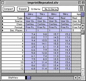
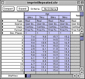
Then click on the "Compact" button to give the set of columns a common name to indicate it is a repeated measure:
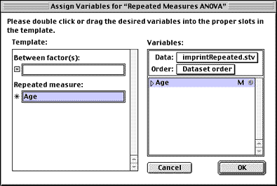
Menu: Analyze > ANOVA and t-tests > Repeated ANOVA
(Note that the "Between Factors" slot is left empty in this case)
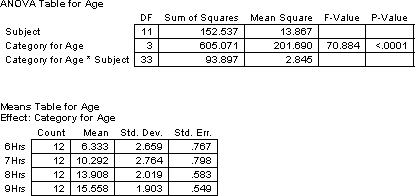
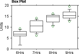

The appropriate statistical test is a within-cases or repeated measures one-way analysis of variance (ANOVA).
To see if newly hatched chicks get better at imprinting (remaining closer to the target for longer times), a group of 12 chicks is tested for 10 minutes at ages 6, 7, 8, and 9 hours. Chicks are placed individually in a box in which a pulley moves a stuffed hen; imprinting scores are assigned based on the distance to the target and the time spent near the target.
| Chick | 6 Hrs | 7 Hrs | 8 Hrs | 9 Hrs |
| 1 | 7.4 | 9.8 | 15.7 | 15.2 |
| 2 | 0.0 | 7.7 | 14.5 | 17.0 |
| 3 | 9.4 | 13.5 | 16.3 | 16.9 |
| 4 | 8.6 | 14.1 | 15.3 | 17.6 |
| 5 | 2.5 | 6.1 | 11.3 | 14.1 |
| 6 | 6.6 | 7.9 | 10.4 | 14.3 |
| 7 | 5.8 | 12.8 | 14.9 | 19.4 |
| 8 | 6.1 | 7.4 | 11.0 | 12.6 |
| 9 | 7.5 | 8.3 | 13.3 | 13.5 |
| 10 | 6.7 | 11.4 | 15.4 | 15.6 |
| 11 | 8.6 | 13.1 | 13.4 | 15.3 |
| 12 | 6.8 | 11.4 | 15.4 | 15.2 |
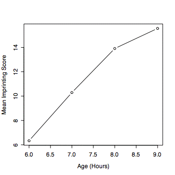
Beginning at six hours old, the mean imprinting scores of 12 chicks significantly increase (F(3,33) = 70.9, p < .0001) with each additional hour of age from 6.3 to 10.3 to 13. 9 to 15.6. Hence, chicks do improve imprinting with practice.
Prepare a csv file like hours.csv
>#read the csv file and examine it
> hrs <- read.csv("hours.csv")
> hrs
   chick hours imprint
1      1     6     7.4
2      1     7     9.8
3      1     8    15.7
4      1     9    15.2
5      2     6     0.0
6      2     7     7.7
7      2     8    14.5
8      2     9    17.0
9      3     6     9.4
10     3     7    13.5
11     3     8    16.3
12     3     9    16.9
13     4     6     8.6
14     4     7    14.1
15     4     8    15.3
16     4     9    17.6
17     5     6     2.5
18     5     7     6.1
19     5     8    11.3
20     5     9    14.1
21     6     6     6.6
22     6     7     7.9
23     6     8    10.4
24     6     9    14.3
25     7     6     5.8
26     7     7    12.8
27     7     8    14.9
28     7     9    19.4
29     8     6     6.1
30     8     7     7.4
31     8     8    11.0
32     8     9    12.6
33     9     6     7.5
34     9     7     8.3
35     9     8    13.3
36     9     9    13.5
37    10     6     6.7
38    10     7    11.4
39    10     8    15.4
40    10     9    15.6
41    11     6     8.6
42    11     7    13.1
43    11     8    13.4
44    11     9    15.3
45    12     6     6.8
46    12     7    11.4
47    12     8    15.4
48    12     9    15.2

> attach(hrs)
>#because the chick id and the IV hours are numbers we convert them to factors
> hours <- factor(hours)
> chick <- factor(chick)
> #examine the means for each hour
> tapply(imprint, hours, mean)
        6         7         8         9
 6.333333 10.291667 13.908333 15.558333

> #do the analysis-of-variance (aov) specifying errors are computed within chicks
> hrs.aov <- aov(imprint ~ hours + Error(chick))
> summary(hrs.aov)

Error: chick
          Df  Sum Sq Mean Sq F value Pr(>F)
Residuals 11 152.537  13.867

Error: Within
          Df Sum Sq Mean Sq F value    Pr(>F)
hours      3 605.07  201.69  70.884 1.806e-14 ***
Residuals 33  93.90    2.85
---
Signif. codes:  0 '***' 0.001 '**' 0.01 '*' 0.05 '.' 0.1 ' ' 1
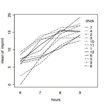
When there are a relativley few cases, as in this instance, it is useful to plot the data for each case. This makes it easy to find cases that do or do not fit the general pattern.
> interaction.plot(hours,chick,imprint)
> #a plot of the means is often useful
> # type="b" plots both points and connecting lines
> plot(c(6,7,8,9),mns,type="b")
Create a dataset like this one and select the columns:

Then click on the "Compact" button to give the set of columns
a common name to indicate it is a repeated measure:

Menu: Analyze > ANOVA and t-tests > Repeated ANOVA
(Note that the "Between Factors" slot is left empty in this case)


In Excel, organize the dataset so that rows correspond to subjects (or whatever is the unit of analysis) and so that columns correspond to the different groups or treatment conditions or time points for the repeated measures. Then use Anova: Two-Factor Without Replication. Ignore the statistical results for the Row. The appropriate F statistic is the one for the Columns.
© 2002, Gary McClelland