www.seeingstatistics.com

Start > Differences > Scores > One IV > Two Groups > Within: Paired t-test

Student's t-test for Paired Groups

The appropriate statistical test is variously called the paired or dependent or within-subjects or within-groups Student t-test. The difference between the paired scores for each case is

These difference scores can then compared against the null hypothesis of zero using the one-sample t-test. An alternative and equivalent formula highlights an important advantage of the paired t-test. With two scores from each of n observations,

where

where r is the correlation between the two sets of scores. Note that the greater the correlation, the smaller is the standard error of the difference, and hence the smaller is the denominator of the t-test. Thus, larger correlations--greater similarity between the scores for each observation--increases the value of the t-statistic.

Example

To evaluate the effectiveness of a computer typing game for improving keyboard skills, 11 third-grade students take a typing test before and after playing the game. To score points in the game, students must correctly type short words to intercept alien invaders on the screen. Scores on the before and after typing test are the number of mistakes made typing matched passages of 30 words.

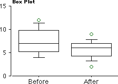
Student	Before	After	Diff
1	8	5	3
2	7	7	0
3	6	4	2
4	12	6	6
5	5	7	-2
6	4	2	2
7	10	7	3
8	9	9	0
9	4	6	-2
10	7	4	3
11	11	7	4
Mean	7.5	5.8	1.7

If playing the typing game had no effect on typing test scores, then we would expect the differences for each student to be zero, on average.

Summary

For 11 third-grade students, the average number of errors on a typing test before playing a computer typing game was 7.5, but after playing the game the average number of errors was 5.8. The reduction of 1.7 errors is statistically significant (t(10) = 2.3, p = .045). Thus, the typing game is effective in improving the keyboard skills of third-grade students.

Computer Examples

R

> before <- c(8,7,6,12,5,4,10,9,4,7,11,7.5)
> after <- c(5,7,4,6,7,2,7,9,6,4,7,5.8)
> mean(before)
[1] 7.541667
> mean(after)
[1] 5.816667
> t.test(after,before,paired=TRUE)

	Paired t-test

data:  after and before 
t = -2.5133, df = 11, p-value = 0.02882
alternative hypothesis: true difference in means is not equal to 0 
95 percent confidence interval:
 -3.2356513 -0.2143487 
sample estimates:
mean of the differences 
                 -1.725 

Alternatively, one may do the one-sample t-test this way:

> t.test(after - before)

	One Sample t-test

data:  after - before 
t = -2.5133, df = 11, p-value = 0.02882
alternative hypothesis: true mean is not equal to 0 
95 percent confidence interval:
 -3.2356513 -0.2143487 
sample estimates:
mean of x 
   -1.725 

#Useful graphs
#boxplot of differences with line indicating 0 change
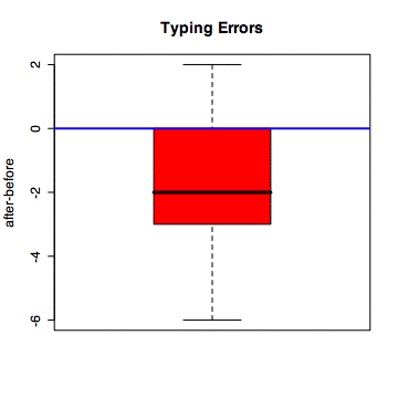
> boxplot(after - before, main="Typing Errors", ylab='after-before', col='red')
> abline(0,0,col='blue', lwd='2')

Advanced

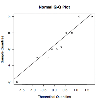
#check assumption of normality
> qqnorm(after - before)
> qqline(after - before)

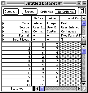
StatView

Prepare a dataset like this one:


/

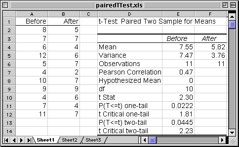
Excel

Menu: Tools > Data Analysis > T-test: Paird Two-Sample for Means

© 2002, Gary McClelland