Menu: Analyze > ANOVA and t-tests > ANOVA or ANCOVA
produces these results:
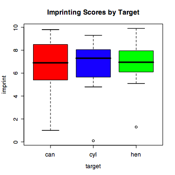
and use Graphs > Boxplot to get this visual comparison:

The appropriate statistical test is a between-cases one-way analysis of variance (ANOVA).
The "genetic template" hypothesis of imprinting posits that ducklings, goslings, chicks, etc. will imprint more strongly to something that resembles a mother duck, gander, or chicken. The alternative hypothesis is that they will imprint to anything that moves. To test this, groups of eight-hour old chicks are placed in a box in which a pulley moves either a stuffed hen, a red watering can, or a yellow cylinder. Imprinting scores are assigned based on the distance to the target and the time spent near the target.
| Group | Imprinting Scores |
| Stuffed Hen |
7.5
7.3
5.1
6.6
6.5
6.6
7.9 8.0 5.7 9.9 1.3 9.0 |
| Watering Can |
6.7
9.4
9.1
1.0
4.9
9.8
7.5 7.9 5.9 6.2 7.1 2.2 |
| Yellow Cylinder |
9.1
4.8
6.3
6.8
5.0
9.3
0.1 7.7 6.9 8.1 8.0 7.9 |
Eight-hour old chicks were not significantly (F(2,33) = 0.05, p = .96) more likely to follow targets genetically similar to hens (mean imprinting score equals 6.8) than they were to follow either a red watering can (6.5) or a yellow cylinder (6.7). Thus, there is no evidence that chicks are born with a genetic template of the target on which they should imprint. Instead, it appears they imprint to whatever object is moving.
Prepare a text file with the values separated by commas as in imprint.csv.
> d <- read.csv('imprint.csv')
> d
   target imprint
1     hen     7.5
2     hen     7.3
3     hen     5.1
4     hen     6.6
5     hen     6.5
6     hen     6.6
7     hen     7.9
8     hen     8.0
9     hen     5.7
10    hen     9.9
11    hen     1.3
12    hen     9.0
13    can     6.7
14    can     9.4
15    can     9.1
16    can     1.0
17    can     4.9
18    can     9.8
19    can     7.5
20    can     7.9
21    can     5.9
22    can     6.2
23    can     7.1
24    can     2.2
25    cyl     9.1
26    cyl     4.8
27    cyl     6.3
28    cyl     6.8
29    cyl     5.0
30    cyl     9.3
31    cyl     0.1
32    cyl     7.7
33    cyl     6.9
34    cyl     8.1
35    cyl     8.0
36    cyl     7.9

> summary(d)
 target      imprint
 can:12   Min.   :0.100
 cyl:12   1st Qu.:5.850
 hen:12   Median :7.000
          Mean   :6.642
          3rd Qu.:8.000
          Max.   :9.900

# get means and standard deviations for each group
# (tapply is "table apply" and applies the specified fnction, in this case
# the mean, to the variable imprint in each group defined by target
> tapply(imprint,target,"mean")
     can      cyl      hen
6.475000 6.666667 6.783333

> tapply(imprint,target,'sd')
     can      cyl      hen
2.716323 2.502120 2.181673

> oneway.test(imprint ~ target, var.equal=TRUE)

	One-way analysis of means

data:  imprint and target
F = 0.0474, num df = 2, denom df = 33, p-value = 0.9537


> plot(imprint ~ target, col=c('red','blue','green'),
+   main='Imprinting Scores by Target')
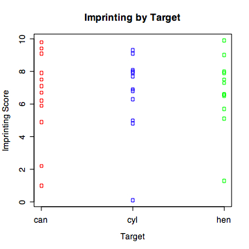
> stripchart(imprint ~ target,vertical=TRUE,col=c('red','blue','green'),
+ ylab='Imprinting Score',xlab='Target',main='Imprinting by Target')
Had there been differences among the groups, the following function is useful for determining which pairs of means are significantly different, adjusting for the fact the multiple comparisons are being conducted on the same dataset.
pairwise.t.test(imprint,target)
#ADVANCED: checking normality of residuals
> gl <- lm(imprint ~ target)
> qqnorm(gl$residuals)
> qqline(gl$residuals, col='blue', lwd=2)
Prepare a dataset like the following. Note that not all the cases are displayed in this image.
Menu: Analyze > ANOVA and t-tests > ANOVA or ANCOVA
produces these results:
and use Graphs > Boxplot to get this visual comparison:
Note: lm() can also be used to perform the one-way anova using indicator variables for levels of the variable. Below is the summary of the lm object created above.
> summary(gl)

Call:
lm(formula = imprint ~ target)

Residuals:
    Min      1Q  Median      3Q     Max
-6.5667 -0.7021  0.3750  1.3562  3.3250

Coefficients:
            Estimate Std. Error t value Pr(>|t|)
(Intercept)   6.4750     0.7149   9.057 1.82e-10 ***
targetcyl     0.1917     1.0110   0.190    0.851
targethen     0.3083     1.0110   0.305    0.762
---
Signif. codes:  0 '***' 0.001 '**' 0.01 '*' 0.05 '.' 0.1 ' ' 1

Residual standard error: 2.476 on 33 degrees of freedom
Multiple R-Squared: 0.002866,	Adjusted R-squared: -0.05757
F-statistic: 0.04742 on 2 and 33 DF,  p-value: 0.9537
Note that the overall F(2,33) = .0474, p = .9537 is exactly the same as reported by the oneway.test() above. In addition, lm() provides R-Squared. To handle the multiple levels of the target variable, lm() constructs indicator variables. The variable targetcyl has the value 1 when the target = cyl and 0 otherwise. Similarly, targethen has the value 1 when the target = hen and 0 otherwise. The intercept is the predicted value when both targetcyl and targethen equal 0, in other words, when target = can. Indeed the estimate of the intercept of 6.475 equals the mean for the can group. The estimate for the targetcyl variable of 0.1917, which is the amount the mean for the cyl group exceeds that of the can group. Similarly, the estimate of 0.3083 for targethen is the amount by which the mean of the hen group exceeds the mean of the can group.
© 2002, Gary McClelland