www.seeingstatistics.com

Start > Differences > Scores > One Group > SD Unknown: One-sample t-test

One-Sample Student's t-test

The appropriate statistical test is the one-sample Student's t-test. The mean of the data are compared to an hypothesized, a priori, or theoretical mean.

The value of t is then compared to the distribution of Student's t with n-1 degrees of freedom.

Example:

Thirteen students keep diaries of their study time. For each student the researcher compuates the ratio of the number of hours studied per each credit hour of classes in which the student is enrolled. The ratios for x students are

   1.9   2.1   1.2   0.7   1.8   1.6   2.4   3.0   0.9   1.3   1.5   1.9   2.0

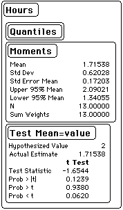
The two-tailed probability of getting a value of t this large or larger with 12 degrees of freedom is 0.1239. Hence, we would not reject the hypothesis that the typical student studied two hours outside of class for each hour in class.

Summary

The mean ratio of out of class study hours to in-class hours for 13 students was 1.7 with a standard deviation of .6. The mean did not differ significantly from the expected ratio of two hours outside class for each hour in class (t(12) = -1.66, p = .12).

Computer Examples

R

# enter the data
> ratio <- c(1.9,2.1,1.2,0.7,1.8,1.6,2.4,3.0,0.9,1.3,1.5,1.9,2.0)

# compute mean and stadard deviation for the data
[1] 0.620277
> mean(ratio)
[1] 1.715385
> sd(ratio)
[1] 0.620277

# perform test, specifying the null hypothesis as mu
> t.test(ratio,mu=2)

	One Sample t-test

data:  ratio 
t = -1.6544, df = 12, p-value = 0.1239
alternative hypothesis: true mean is not equal to 2 
95 percent confidence interval:
 1.340555 2.090214 
sample estimates:
mean of x 
 1.715385 

#construct a boxplot
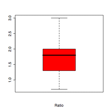
boxplot(ratio, col="red", xlab="Ratio")

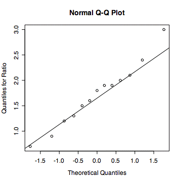
#ADVANCED:  Checking assumption of normal distribution
# If observations are from normal distribution, they will be more or less
# on the line in the quantile-quantile graph
> qqnorm(ratio,ylab="Quantiles for Ratio")
> qqline(ratio)

Statview

Jmp

Minitab

MTB > TTest 2 'Hours';
SUBC>   Alternative 0.

T-Test of the Mean


Test of mu = 2.000 vs mu not = 2.000

Variable     N      Mean    StDev   SE Mean        T    P-Value
Hours       13     1.715    0.620     0.172    -1.65       0.12

Excel

Excel will not directly perform this statistical test with the tools available in the Data Analysis toolpack. Click to download ttestOneSample.xls, an Excel worksheet that will perform the t-test for the mean when the variance is unknown.

© 2002, Gary McClelland