www.seeingstatistics.com

Start > Relationship > Score > One IV

Simple Regression

The appropriate statistical procedure is simple regression. The correlation coefficient is also appropriate (and is closely related to regression). Simple regression estimates coefficients a (intercept) and b (slope) for the best-fitting line relating X to Y. That is,



and provides tests of whether those coefficients are significantly different from zero.

Example

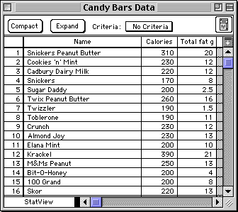
StatView is distributed with a sample dataset containing information about various canday bars. Suppose we wanted to know whether the total grams of Fat (per serving size) predicted the number of Calories (per serving size). See the StatView computer example below for an extract from the dataset.

Summary

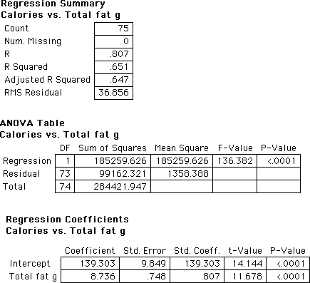
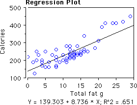
The higher the total grams of fat in a candy bar's serving size, the higher the number of calories per serving size (t(73) = 11.7, p < .0001). Each additional gram of fat adds about 8.7 calories and candy bars with no fat have about 140 calories. The correlation between grams of fat and calories is .81 or about 65% of the variation in calories is predicted by grams of fat.

Computer Examples

R

This example below assumes the variables are already available in a dataset candy. To enter data directly, use:

x <- c(1,1,2,2,3,3,4,4,5,5,6,6,7,7,8,8)

attach(candy)
#compute the correlation coefficient
> cor(calories,totalFat)
[1] 0.8070656

#test whether the correlation coefficient differs from 0
> cor.test(calories, totalFat)

	Pearson's product-moment correlation

data:  calories and totalFat 
t = 11.6783, df = 73, p-value < 2.2e-16
alternative hypothesis: true correlation is not equal to 0 
95 percent confidence interval:
 0.7101918 0.8739444 
sample estimates:
      cor 
0.8070656 

#do the regression and save it as an object
candyLM <- lm(calories ~ totalFat)
#use summary() to extract the basic information
> summary(candyLM)

Call:
lm(formula = calories ~ totalFat)

Residuals:
   Min     1Q Median     3Q    Max 
-49.19 -29.71 -12.87  27.65  88.86 

Coefficients:
            Estimate Std. Error t value Pr(>|t|)    
(Intercept)  139.303      9.849   14.14   <2e-16 ***
totalFat       8.736      0.748   11.68   <2e-16 ***
---
Signif. codes:  0 Ô***Õ 0.001 Ô**Õ 0.01 Ô*Õ 0.05 Ô.Õ 0.1 Ô Õ 1 

Residual standard error: 36.86 on 73 degrees of freedom
Multiple R-Squared: 0.6514,	Adjusted R-squared: 0.6466 
F-statistic: 136.4 on 1 and 73 DF,  p-value: < 2.2e-16 

#examine scatterplot 
plot(calories ~ totalFat)
#add the regression line to the plot
abline(candyLM)

Example Entering Data Directly

In a study to determine whether the number of exposures to a set of words was related to the number of words recalled in a test an hour later, students were randomly assigned to experience 1, 2, 3, 4, 5, 6, 7, or 8 exposures. The data are shown in the commands below.

> #enter the data for each variable, being careful that corresponding entries for each variable
> #are from the same student.
> recall <- c(4,3,3,5,6,4,4,6,5,7,2,9,6,8,9,8)
> expose <- c(1,1,2,2,3,3,4,4,5,5,6,6,7,7,8,8)

> wordLM <- lm(recall ~ expose)
> summary(wordLM)

Call:
lm(formula = recall ~ expose)

Residuals:
    Min      1Q  Median      3Q     Max 
-4.5000 -0.9062  0.4375  1.0312  2.5000 

Coefficients:
            Estimate Std. Error t value Pr(>|t|)   
(Intercept)   2.7500     0.9211   2.986  0.00983 **
expose        0.6250     0.1824   3.427  0.00409 **
---
Signif. codes:  0 Ô***Õ 0.001 Ô**Õ 0.01 Ô*Õ 0.05 Ô.Õ 0.1 Ô Õ 1 

Residual standard error: 1.672 on 14 degrees of freedom
Multiple R-Squared: 0.4561,	Adjusted R-squared: 0.4173 
F-statistic: 11.74 on 1 and 14 DF,  p-value: 0.004091 

StatView

Extract from the dataset:



Menu: Analyze > Regression > Regression--Simple

© 2002, Gary McClelland